You are employed by a modern insurance company that markets term insurance to clients through a variety of outreach techniques. Although they might be quite expensive, telephone marketing initiatives remain one of the best ways to connect with potential customers. Therefore, in order to carefully target these clients with phone calls, it is imperative to identify those who are most likely to convert beforehand. Using the company’s past marketing data, our goal is to create a machine learning model that can forecast whether a customer would sign up for insurance. We are going to build customer conversion prediction model classification analysis.
So It’s a classification problem. We will apply following machine learning algorithms
- Logistic Regression
- Decision Tree Classifier
- Random Forest Classifier
- K-Nearest Neighbor
- XG Boost
Dataset can be download from kaggle. Here the link of dataset Customer Conversion Prediction.
Columns info

customer_dt.isnull().sum()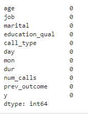
customer_dt.describe()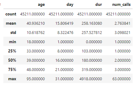
#checking for the data is balanced or not
customer_dt['y'].value_counts()
len(customer_dt)45211
# Calculate the value counts for each class
value_counts = customer_dt['y'].value_counts()

# Calculate the percentage for each class
percentage = value_counts / len(customer_dt) * 100

# Display the percentage
print(percentage)
Finding Duplicate values
customer_dt.duplicated().sum()6
# We will remove duplicate values

customer_dt = customer_dt.drop_duplicates()customer_dt.info()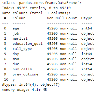
Unique values of categorical columns
# Loop through each column in the DataFrame
for column in customer_dt.columns:
    # Check if the column is of object type (categorical)
    if customer_dt[column].dtype == 'object':
        # Print the unique values for the categorical column
        print(f"Unique values in '{column}': {customer_dt[column].unique()}")
        print("-" * 50)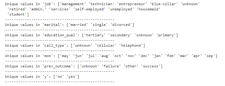
Explore this dataset and replace unknown values
customer_dt.job.value_counts()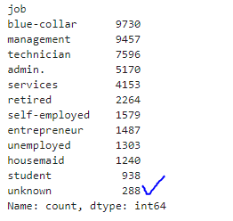
len(customer_dt)45205
Therefore, of the 45205 rows in the dataset, 288 values are unknown in the job variable; thus, removing 288 rows will not have a greater impact on the dataset.
#replacing unknown value as null
customer_dt.loc[customer_dt['job'] == 'unknown', 'job'] = np.nan
customer_dt.isnull().sum()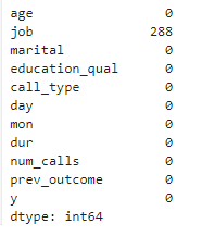
customer_dt = customer_dt.dropna(subset = ['job'])
customer_dt.isnull().sum()
len(customer_dt)44917
customer_dt.education_qual.value_counts()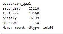
# Calculate the total number of entries in the education_qual column
total_entries = customer_dt['education_qual'].count()

# Calculate the number of 'unknown' entries in the education_qual column
unknown_count = customer_dt['education_qual'].value_counts()['unknown']

# Calculate the percentage of 'unknown' values
unknown_percentage = (unknown_count / total_entries) * 100

# Print the result
print(f"Percentage of 'unknown' in education_qual: {unknown_percentage:.2f}%")
Percentage of 'unknown' in education_qual: 3.85%
Since there is 3.85% of unknown in education_qual, we will eliminate it since it has no bearing on the dataset.
# Remove rows where 'education_qual' is 'unknown'
customer_dt = customer_dt[customer_dt['education_qual'] != 'unknown']
len(customer_dt)
43187
customer_dt.call_type.value_counts()
# Calculate the total number of entries in the call_type column
total_entries_cl = customer_dt['call_type'].count()

# Calculate the number of 'unknown' entries in the call_type column
unknown_count_cl = customer_dt['call_type'].value_counts()['unknown']

# Calculate the percentage of 'unknown' values
unknown_percentage_cl = (unknown_count_cl / total_entries_cl) * 100

# Print the result
print(f"Percentage of 'unknown' in call_type: {unknown_percentage_cl:.2f}%")
Percentage of 'unknown' in call_type: 28.44%
Since there is 28.44 percent of unknown in call_type, we shall keep it.
customer_dt.prev_outcome.value_counts()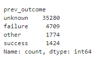
# Calculate the total number of entries in the prev_outcome column
total_entries_pr = customer_dt['prev_outcome'].count()

# Calculate the number of 'unknown' entries in the prev_outcome column
unknown_count_pr = customer_dt['prev_outcome'].value_counts()['unknown']

# Calculate the percentage of 'unknown' values
unknown_percentage_pr = (unknown_count_pr / total_entries_pr) * 100

# Print the result
print(f"Percentage of 'unknown' in prev_outcome: {unknown_percentage_pr:.2f}%")
Percentage of 'unknown' in prev_outcome: 81.69%
Since there is 81.69 percent of unknown in prev_outcome, we shall keep it.
Outlier detection and removal
# Show the boxplot of age
plt.figure(figsize=(10, 6))
sns.boxplot(x=customer_dt['age'])
plt.title('Boxplot of Age')
plt.xlabel('Age')
plt.show()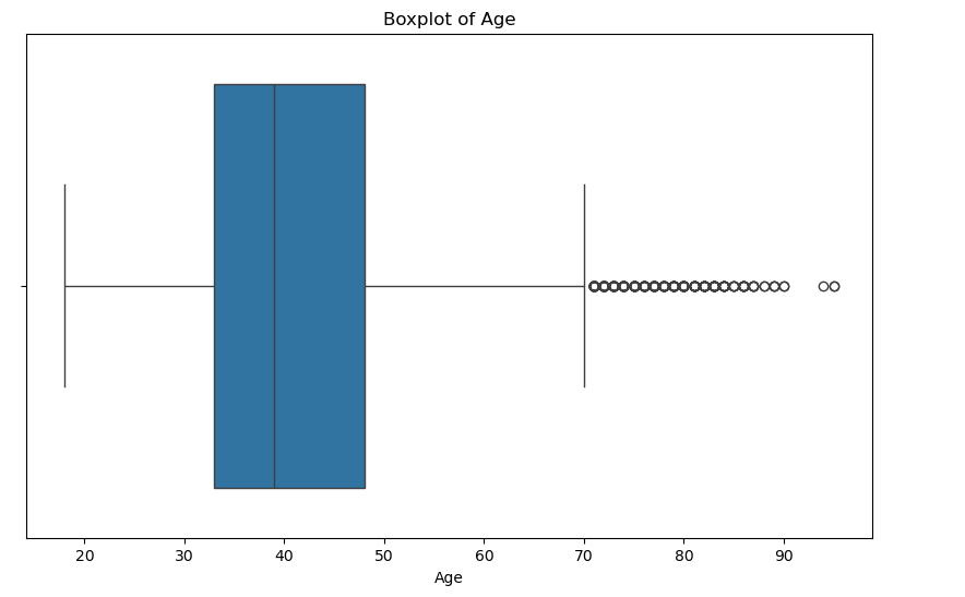
# Calculate the IQR for age
Q1_g = customer_dt['age'].quantile(0.25)
Q3_g = customer_dt['age'].quantile(0.75)
IQR_g = Q3_g - Q1_g

# Determine the lower and upper bounds for outliers
lower_bound_g = Q1_g - 1.5 * IQR_g
upper_bound_g = Q3_g + 1.5 * IQR_g

print(f"Lower Bound of age column: {lower_bound_g}")
print(f"Upper Bound of age column: {upper_bound_g}")

# Identify outliers
outliers_g = customer_dt[(customer_dt['age'] < lower_bound_g) | (customer_dt['age'] > upper_bound_g)]


# Count the number of outliers
num_outliers_g = outliers_g.shape[0]
print(f"Number of outliers in the 'age' column: {num_outliers_g}")

outliers_g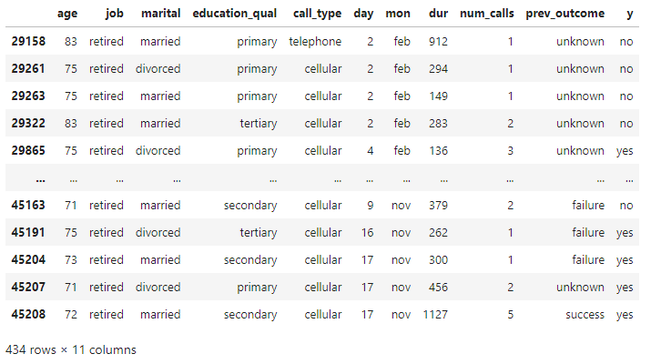
customer_dt = customer_dt[(customer_dt['age'] >= lower_bound_g) & (customer_dt['age'] <= upper_bound_g)]
customer_dt.shape
(42753, 11)
Again check box plot of age
# Show the boxplot of age
plt.figure(figsize=(10, 6))
sns.boxplot(x=customer_dt['age'])
plt.title('Boxplot of Age')
plt.xlabel('Age')
plt.show()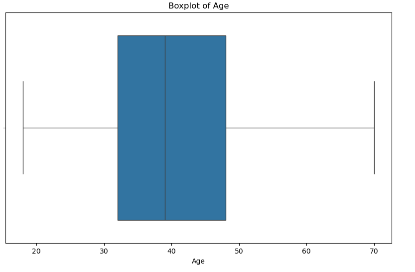
# Show the boxplot of day
plt.figure(figsize=(10, 6))
sns.boxplot(x=customer_dt['day'])
plt.title('Boxplot of Day')
plt.xlabel('Day')
plt.show()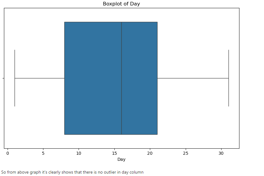
# Show the boxplot of dur
plt.figure(figsize=(10, 6))
sns.boxplot(x=customer_dt['dur'])
plt.title('Boxplot of Duration')
plt.xlabel('Duration')
plt.show()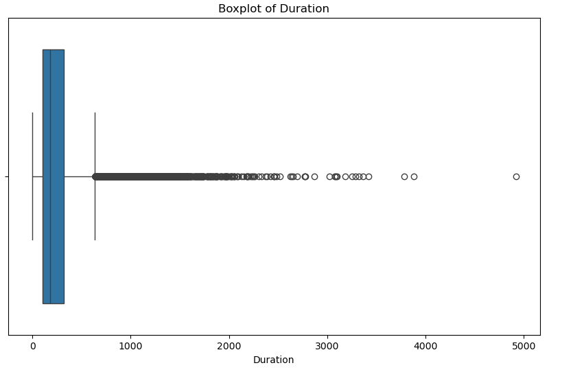
# Calculate the IQR for duration
Q1_dur = customer_dt['dur'].quantile(0.25)
Q3_dur = customer_dt['dur'].quantile(0.75)
IQR_dur = Q3_dur - Q1_dur

# Determine the lower and upper bounds for outliers
lower_bound_dur = Q1_dur - 1.5 * IQR_dur
upper_bound_dur = Q3_dur + 1.5 * IQR_dur


# Identify outliers
outliers_dur = customer_dt[(customer_dt['dur'] < lower_bound_dur) | (customer_dt['dur'] > upper_bound_dur)]


# Count the number of outliers
num_outliers_dur = outliers_dur.shape[0]
print(f"Number of outliers in the 'durarion' column: {num_outliers_dur}")
Number of outliers in the 'durarion' column: 3093
outliers_dur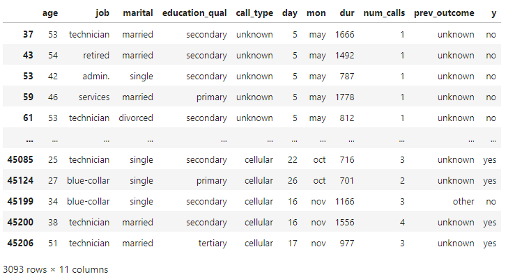
customer_dt = customer_dt[(customer_dt['dur'] >= lower_bound_dur) & (customer_dt['dur'] <= upper_bound_dur)]
customer_dt.shape
(39660, 11)
# Show the boxplot of dur
plt.figure(figsize=(10, 6))
sns.boxplot(x=customer_dt['dur'])
plt.title('Boxplot of Duration')
plt.xlabel('Duration')
plt.show()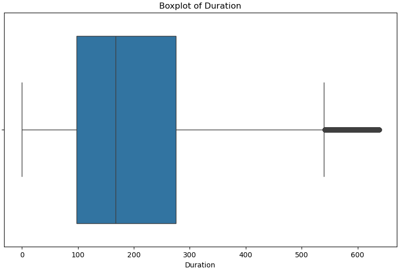
# Show the boxplot of dur
plt.figure(figsize=(10, 6))
sns.boxplot(x=customer_dt['num_calls'])
plt.title('Boxplot of Number of Calls')
plt.xlabel('Number of Calls')
plt.show()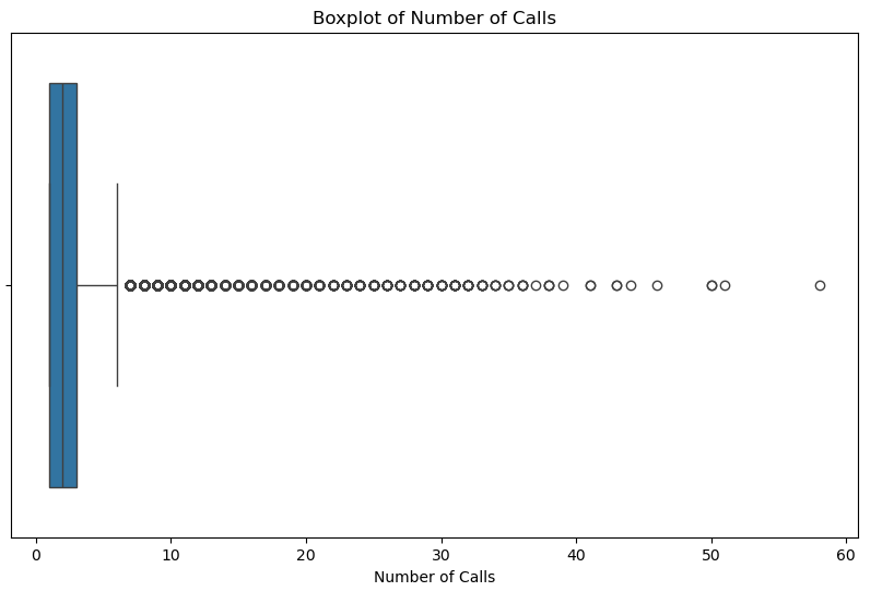
# Calculate the IQR for age
Q1_cl = customer_dt['num_calls'].quantile(0.25)
Q3_cl = customer_dt['num_calls'].quantile(0.75)
IQR_cl = Q3_cl - Q1_cl

# Determine the lower and upper bounds for outliers
lower_bound_cl = Q1_cl - 1.5 * IQR_cl
upper_bound_cl = Q3_cl + 1.5 * IQR_cl

print(f"Lower Bound of num_calls column: {lower_bound_cl}")
print(f"Upper Bound of num_calls column: {upper_bound_cl}")

# Identify outliers
outliers_cl = customer_dt[(customer_dt['num_calls'] < lower_bound_cl) | (customer_dt['num_calls'] > upper_bound_cl)]


# Count the number of outliers
num_outliers_cl = outliers_cl.shape[0]
print(f"Number of outliers in the 'age' column: {num_outliers_cl}")
Lower Bound of num_calls column: -2.0 Upper Bound of num_calls column: 6.0 Number of outliers in the 'age' column: 2720
outliers_cl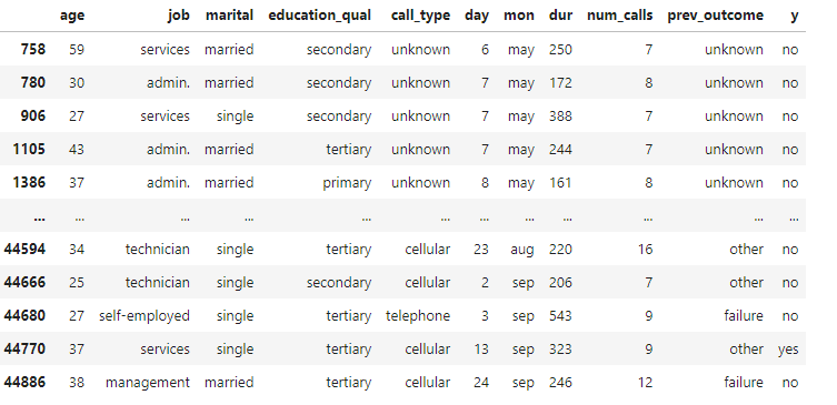
customer_dt = customer_dt[(customer_dt['num_calls'] >= lower_bound_cl) & (customer_dt['num_calls'] <= upper_bound_cl)]
customer_dt.shape
(36940, 11)
# Show the boxplot of dur
plt.figure(figsize=(10, 6))
sns.boxplot(x=customer_dt['num_calls'])
plt.title('Boxplot of Number of Calls')
plt.xlabel('Number of Calls')
plt.show()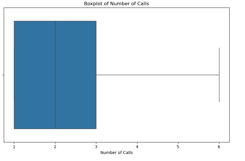
Exploratory Data Analysis
Distribution of Target Variable y
sns.countplot(x = 'y', data = customer_dt)
plt.title('Distribution of Output variable y')
plt.show()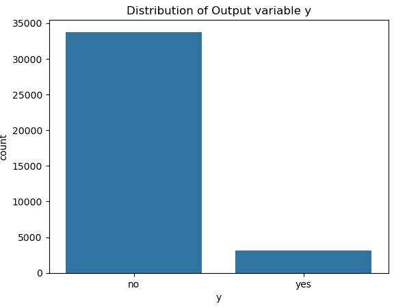
y = customer_dt['y'].value_counts()
plt.pie(y.values,
        labels=y.index,
        autopct='%1.1f%%')
plt.show()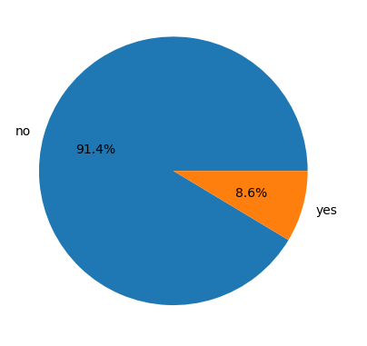
Numerical Columns Distribution
# Plot histograms for numerical features
customer_dt.hist(bins=20, figsize=(14,10))
plt.show()

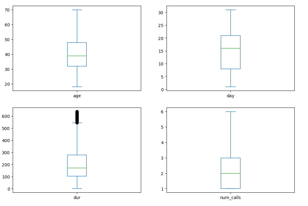
# Boxplot for numerical features
customer_dt[['age', 'day', 'dur', 'num_calls']].plot(kind='box', subplots=True, layout=(2,2), figsize=(12,8))
plt.show()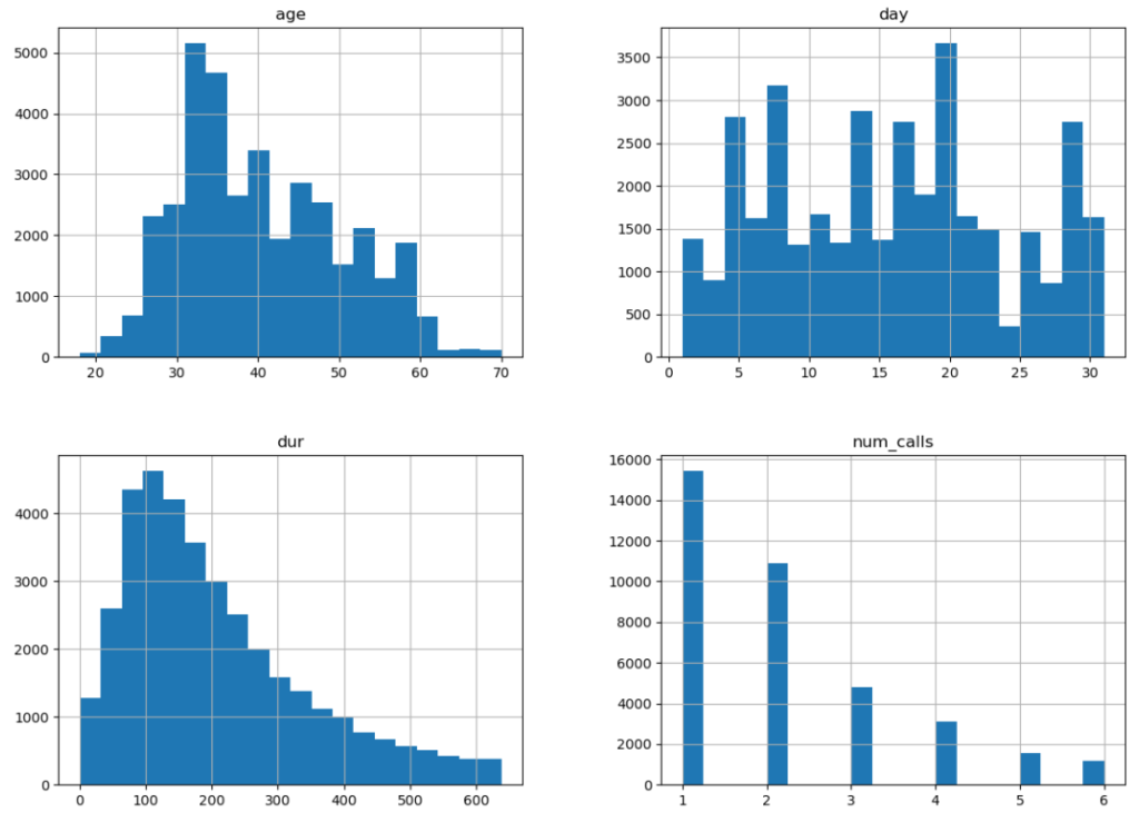
Distribution of Categorical Variables
# List of categorical features
categorical_features = ['job', 'marital', 'education_qual', 'call_type', 'mon', 'prev_outcome']

# Set up a 3x2 grid for plotting
fig, axes = plt.subplots(3, 2, figsize=(15, 15))

# Flatten the axes array for easy iteration
axes = axes.flatten()

# Loop through the categorical features and create count plots
for i, column in enumerate(categorical_features):
    sns.countplot(x=column, data=customer_dt, ax=axes[i])
    axes[i].set_title(f'Distribution of {column}')
    axes[i].set_ylabel('Count')
    axes[i].set_xlabel(column)
    axes[i].tick_params(axis='x', rotation=45)

# Adjust layout for better spacing
plt.tight_layout()
plt.show()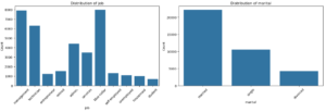


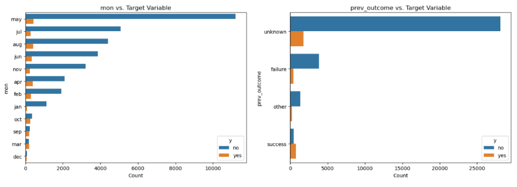
Categorical features vs Target (Outcome)
# List of categorical features to plot
categorical_features = ['job', 'marital', 'education_qual', 'call_type', 'mon', 'prev_outcome']

# Set up a 3x2 grid for plotting
fig, axes = plt.subplots(3, 2, figsize=(15, 15))

# Flatten the axes array for easy iteration
axes = axes.flatten()

# Loop through the categorical features and create count plots
for i, column in enumerate(categorical_features):
    sns.countplot(y=column, hue='y', data=customer_dt, order=customer_dt[column].value_counts().index, ax=axes[i])
    axes[i].set_title(f'{column} vs. Target Variable')
    axes[i].set_xlabel('Count')
    axes[i].set_ylabel(column)

# Adjust layout for better spacing
plt.tight_layout()
plt.show()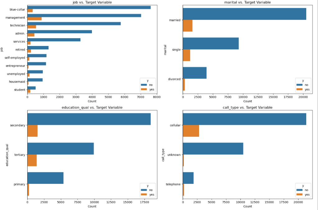
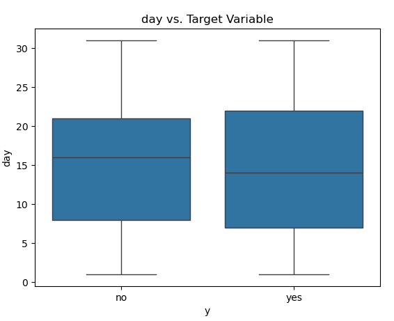
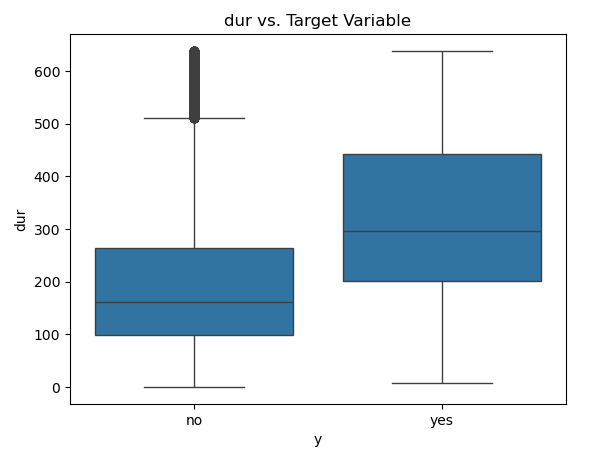
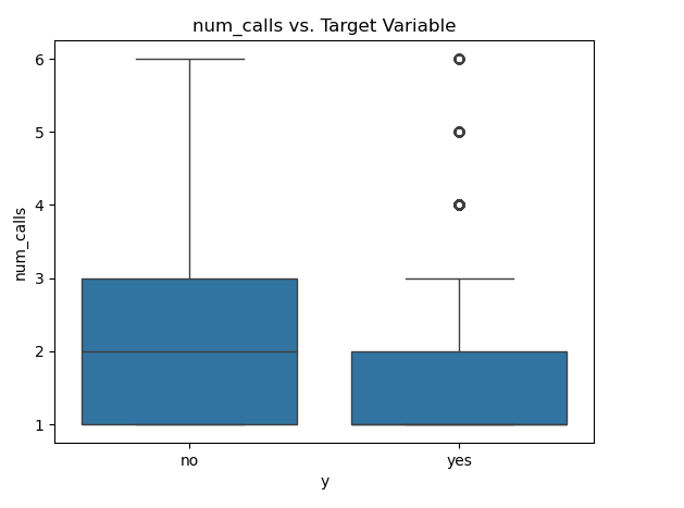
Numeric features vs Target (Outcome)
# Boxplot to see the relationship between numerical features and target variable
for column in ['age', 'day', 'dur', 'num_calls']:
    sns.boxplot(x='y', y=column, data=customer_dt)
    plt.title(f'{column} vs. Target Variable')
    plt.show()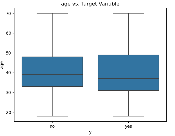
Correlation Analysis
# Select only numeric columns
numeric_cols = customer_dt.select_dtypes(include=['int64', 'float64'])

# Compute the correlation matrix
corr_matrix = numeric_cols.corr()

# Plot the heatmap
plt.figure(figsize=(10, 8))
sns.heatmap(corr_matrix, annot=True, cmap='coolwarm')
plt.title('Correlation Matrix')
plt.show()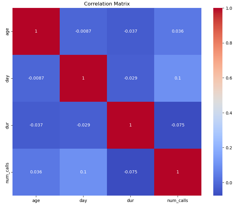
Encoding and Train test splitting the dataset
# Label encode the targer variable Y

from sklearn.preprocessing import LabelEncoder
le = LabelEncoder()
customer_dt['y'] = le.fit_transform(customer_dt['y'])
X = customer_dt.drop(columns = ['y'])
y = customer_dt['y']#Split data into training and testing
from sklearn.model_selection import train_test_split
X_train, X_test, y_train, y_test = train_test_split(X, y, test_size = 0.2 , random_state = 42)Ordinal and Nominal Encoding
# List the columns that need to be transformed
ordinal_features = ['education_qual']
nominal_features = ['job', 'marital', 'call_type', 'mon', 'prev_outcome']
# Define the transformers
from sklearn.compose import ColumnTransformer
from sklearn.preprocessing import OrdinalEncoder, OneHotEncoder, StandardScaler
preprocessor = ColumnTransformer(
    transformers=[
        ('ord', OrdinalEncoder(categories=[['primary', 'secondary', 'tertiary']]), ordinal_features),
        ('nom', OneHotEncoder(drop='first', sparse_output=False), nominal_features)
    ],
    remainder='passthrough'  # This will leave the numeric features as they are
)
# Apply the ColumnTransformer to the training data
X_train_processed = preprocessor.fit_transform(X_train)
X_test_processed = preprocessor.transform(X_test)scaler = StandardScaler()# Identify where numeric columns start after transformation
# The ordinal encoding adds 1 column, and one-hot encoding adds columns equal to the number of unique values in the nominal features minus one for each.
ordinal_columns = 1 # Only 1 ordinal feature 'education_qual'
onehot_columns = sum(len(preprocessor.transformers_[1][1].categories_[i]) - 1 for i in range(len(preprocessor.transformers_[1][1].categories_)))
num_start = ordinal_columns + onehot_columns# Scale only the numeric features
X_train_scaled_numeric = scaler.fit_transform(X_train_processed[:, num_start:])
X_test_scaled_numeric = scaler.transform(X_test_processed[:, num_start:])# Combine scaled numeric features with encoded categorical features
X_train_final = np.hstack((X_train_processed[:, :num_start], X_train_scaled_numeric))
X_test_final = np.hstack((X_test_processed[:, :num_start], X_test_scaled_numeric))Applying Logistic Regression
from sklearn.linear_model import LogisticRegression
#  Train the Logistic Regression model
modelLg = LogisticRegression()
modelLg.fit(X_train_final, y_train)
# Predict on the test data
y_predLg = modelLg.predict(X_test_final)
# Evaluate the model
from sklearn.metrics import accuracy_score, confusion_matrix, classification_report
accuracy = accuracy_score(y_test, y_predLg)
print(f'Accuracy: {accuracy:.2f}')Accuracy: 0.93
conf_matrix = confusion_matrix(y_test, y_predLg)
print('Confusion Matrix:')
print(conf_matrix)
Confusion Matrix: [[6692 94] [ 441 161]]
class_report = classification_report(y_test, y_predLg)
print('Classification Report:')
print(class_report)
Classification Report:
precision recall f1-score support
0 0.94 0.99 0.96 6786
1 0.63 0.27 0.38 602
accuracy 0.93 7388
macro avg 0.78 0.63 0.67 7388
weighted avg 0.91 0.93 0.91 7388
# Logistic Regression Predictions

sns.scatterplot(x=y_test, y=y_predLg, hue=y_predLg, palette='viridis', alpha=0.7, edgecolor=None)
plt.title('Logistic Regression Predictions')
plt.xlabel('True Values')
plt.ylabel('Predicted Values')
plt.grid(True)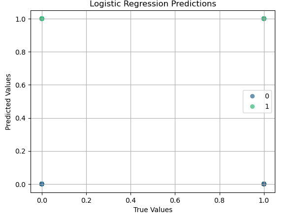
K-Nearest Neighbor (KNN)
from sklearn.neighbors import KNeighborsClassifier
# Initialize a list to store accuracy scores for each value of n_neighbors
accuracy_scores = []

# Manually try different values of n_neighbors
for k in range(1, 21):  # Trying values from 1 to 20
    knn_model = KNeighborsClassifier(n_neighbors=k)
    knn_model.fit(X_train_final, y_train)  # Train the model
    y_pred = knn_model.predict(X_test_final)  # Predict on the test set
    accuracy = accuracy_score(y_test, y_pred)  # Calculate accuracy
    accuracy_scores.append(accuracy)  # Store the accuracy

# Plot the accuracy scores
plt.figure(figsize=(10, 6))
plt.plot(range(1, 21), accuracy_scores, marker='o', linestyle='-', color='b')
plt.title('Accuracy vs. Number of Neighbors (K)')
plt.xlabel('Number of Neighbors (K)')
plt.ylabel('Accuracy')
plt.xticks(range(1, 21))
plt.grid(True)
plt.show()

# Identify the best k
best_k = accuracy_scores.index(max(accuracy_scores)) + 1
best_accuracy = max(accuracy_scores)

print(f'Best number of neighbors: {best_k}')
print(f'Best accuracy: {best_accuracy:.4f}')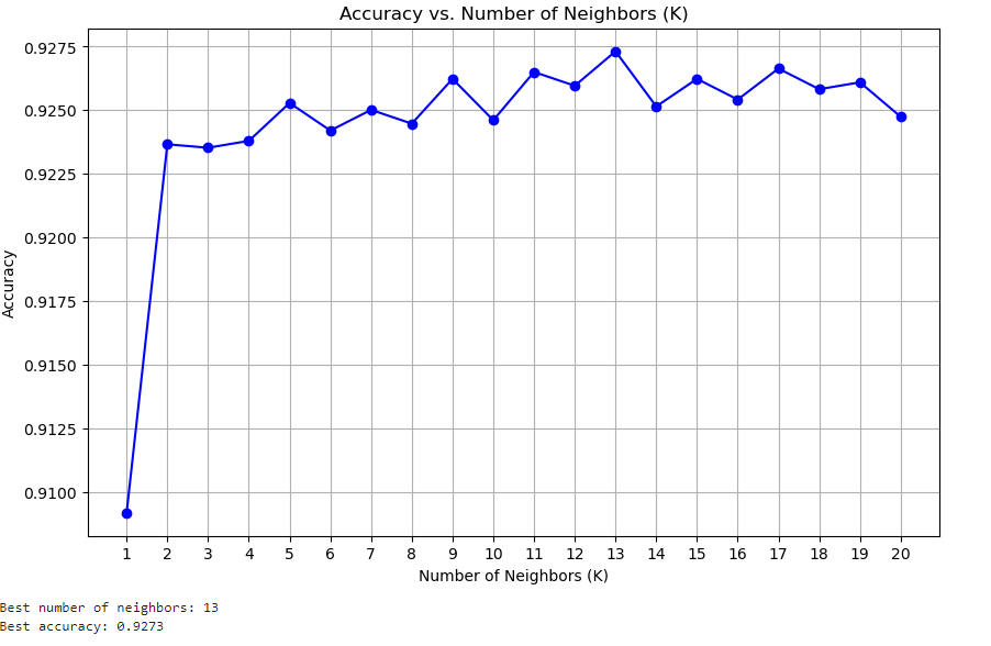
Decision Tree Classifier
from sklearn.tree import DecisionTreeClassifier, plot_tree
# Initialize and train the Decision Tree model
decision_tree_model = DecisionTreeClassifier(random_state=42)
decision_tree_model.fit(X_train_final, y_train)

# Make predictions on the test set
y_pred_tree = decision_tree_model.predict(X_test_final)

# Evaluate the model
accuracy_tree = accuracy_score(y_test, y_pred_tree)
print(f'Accuracy of Decision Tree: {accuracy_tree:.4f}')
Accuracy of Decision Tree: 0.9004
# Create confusion matrix
conf_matrix_tree = confusion_matrix(y_test, y_pred_tree)
conf_matrix_tree
array([[6386, 400],
[ 336, 266]], dtype=int64)
# Plot decision tree
plt.figure(figsize=(20, 10))
plot_tree(decision_tree_model, feature_names=preprocessor.get_feature_names_out(), class_names=['no', 'yes'], filled=True)
plt.title('Decision Tree Visualization')
plt.show()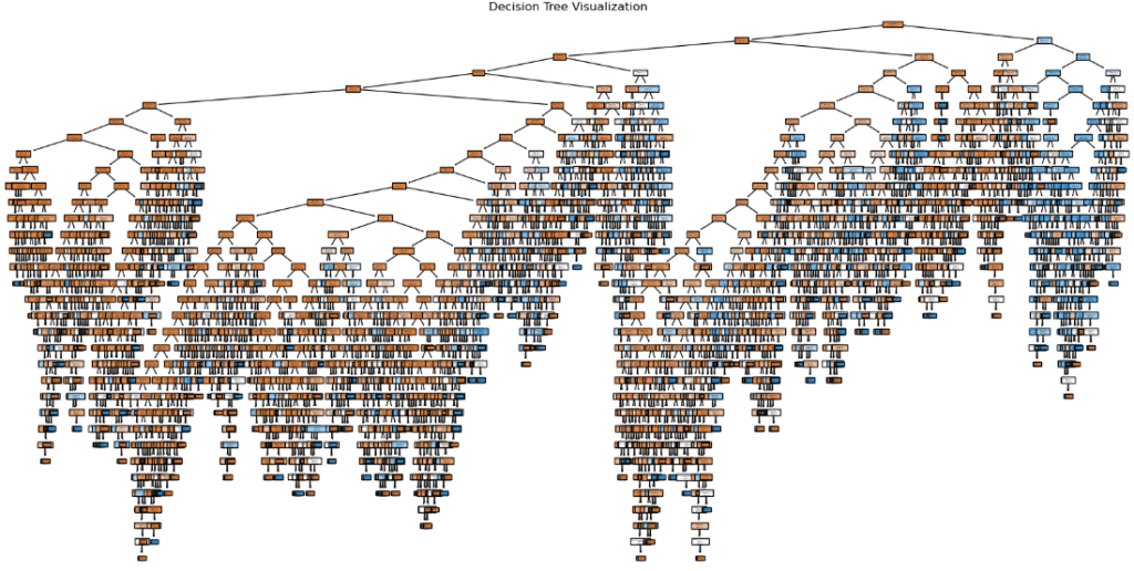
XGB Classifier
import xgboost as xgb
# Initialize and train the XGBoost model
xgb_model = xgb.XGBClassifier(eval_metric='logloss',  random_state=42)
xgb_model.fit(X_train_final, y_train)
# Make predictions on the test set
y_pred_xgb = xgb_model.predict(X_test_final)

# Evaluate the model
accuracy_xgb = accuracy_score(y_test, y_pred_xgb)
print(f'Accuracy of XGBoost: {accuracy_xgb:.4f}')
Accuracy of XGBoost: 0.9285
# Plot feature importances
plt.figure(figsize=(12, 8))
xgb.plot_importance(xgb_model, importance_type='weight', title='Feature Importances', xlabel='Feature Importance', ylabel='Features')
plt.show()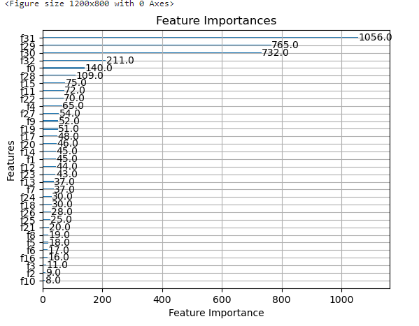
Random Forest Classifier
from sklearn.ensemble import RandomForestClassifier
# Initialize and train the Random Forest model
random_forest_model = RandomForestClassifier(n_estimators=100, random_state=42)
random_forest_model.fit(X_train_final, y_train)

# Make predictions on the test set
y_pred_rf = random_forest_model.predict(X_test_final)

# Evaluate the model
accuracy_rf = accuracy_score(y_test, y_pred_rf)
print(f'Accuracy of Random Forest: {accuracy_rf:.4f}')
Accuracy of Random Forest: 0.9327
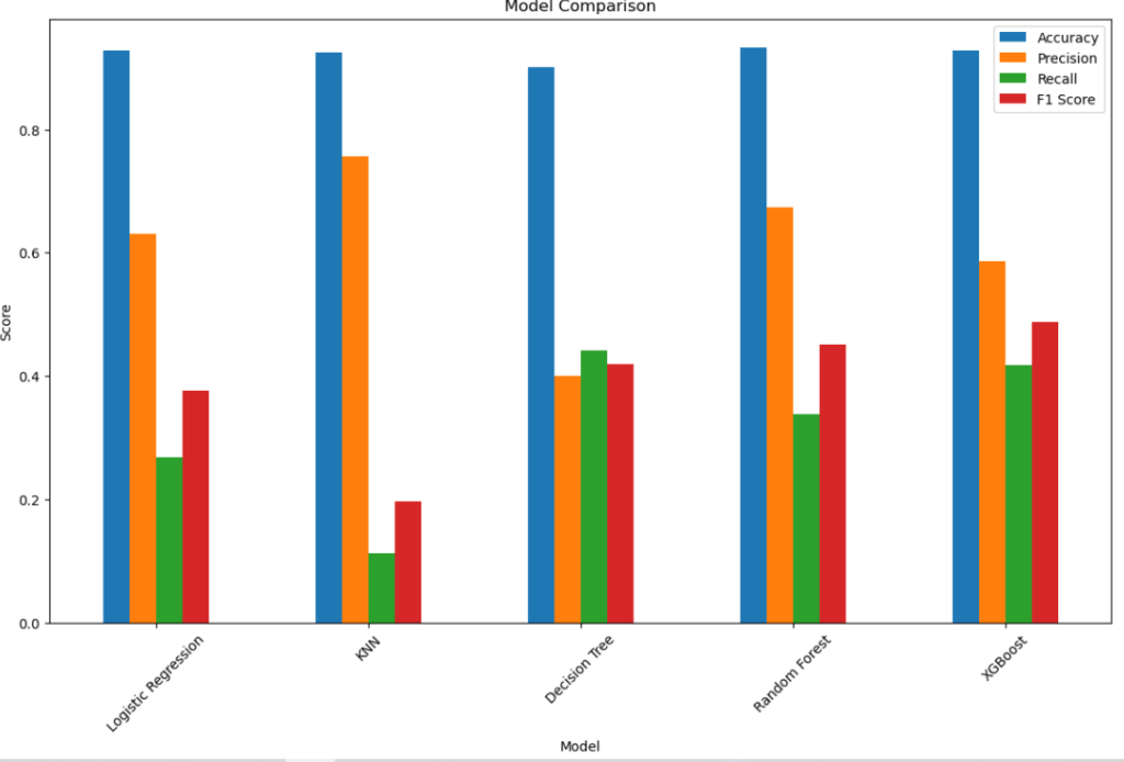
Comparing the models and check which one best
from sklearn.metrics import accuracy_score, precision_score, recall_score, f1_score, classification_report
# Evaluate models
metrics = {
    'Model': ['Logistic Regression', 'KNN', 'Decision Tree', 'Random Forest', 'XGBoost'],
    'Accuracy': [
        accuracy_score(y_test, y_predLg),
        accuracy_score(y_test, y_pred),
        accuracy_score(y_test, y_pred_tree),
        accuracy_score(y_test, y_pred_rf),
        accuracy_score(y_test, y_pred_xgb),
    ],
    'Precision': [
        precision_score(y_test, y_predLg, pos_label= 1),
        precision_score(y_test, y_pred, pos_label=1),
        precision_score(y_test, y_pred_tree, pos_label=1),
        precision_score(y_test, y_pred_rf, pos_label=1),
        precision_score(y_test, y_pred_xgb, pos_label=1),
    ],
    'Recall': [
        recall_score(y_test, y_predLg, pos_label=1),
        recall_score(y_test, y_pred, pos_label=1),
        recall_score(y_test, y_pred_tree, pos_label=1),
        recall_score(y_test, y_pred_rf, pos_label=1),
        recall_score(y_test, y_pred_xgb, pos_label=1),
    ],
    'F1 Score': [
        f1_score(y_test, y_predLg, pos_label=1),
        f1_score(y_test, y_pred, pos_label=1),
        f1_score(y_test, y_pred_tree, pos_label=1),
        f1_score(y_test, y_pred_rf, pos_label=1),
        f1_score(y_test, y_pred_xgb, pos_label=1),
    ]
}
# Create DataFrame for better visualization
metrics_df = pd.DataFrame(metrics)

# Display metrics
print(metrics_df)

# Plot metrics for comparison
metrics_df.set_index('Model').plot(kind='bar', figsize=(14, 8))
plt.title('Model Comparison')
plt.ylabel('Score')
plt.xlabel('Model')
plt.xticks(rotation=45)
plt.legend(loc='best')
plt.show()
                 Model  Accuracy  Precision    Recall  F1 Score
0  Logistic Regression  0.927585   0.631373  0.267442  0.375729
1                  KNN  0.924743   0.755556  0.112957  0.196532
2        Decision Tree  0.900379   0.399399  0.441860  0.419558
3        Random Forest  0.932729   0.673267  0.338870  0.450829
4              XGBoost  0.928533   0.586449  0.416944  0.487379
