Bike Sharing demand prediction regression problem

Bike sharing systems represent a new wave of bicycle rentals where membership, rental, and return are all handled automatically. These systems make it simple for users to borrow a bike from one location and drop it off at another. There are currently more than 500 bike-sharing schemes operating worldwide, with over 500 thousand bicycles. These systems are of tremendous interest now because of their significance in relation to transportation, environmental, and health issues. Here we will perform bike sharing demand prediction by using regression machine learning algorithms.

Bike sharing systems are desirable for research due to their data generation qualities, in addition to their intriguing real-world applications. In contrast to other modes of transportation like buses and subways, these systems openly record the length of journey as well as the position of departure and arrival. With the help of this function, the bike sharing system becomes a virtual sensor network that can be utilized to monitor urban transportation. Therefore, it is anticipated that most significant occurrences in the city could be found by keeping an eye on these data.

It’s a regression problem. We will apply following machine learning projects and at the end of this we will compare all these machine learning algorithms.

Linear Regression
Support Vector Regressor
Decision Tree Regressor
Random Forest Regressor
Gradient Boosting Regressor

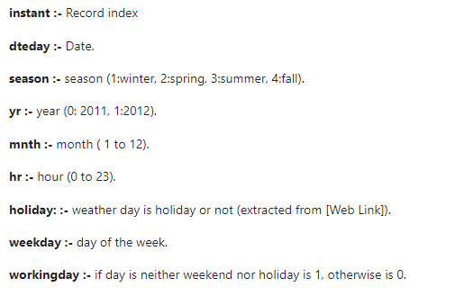
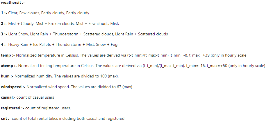
Columns info

Importing required libraries

#imporing required libraries
import numpy as np
import pandas as pd
import matplotlib.pyplot as plt
import seaborn as sns
from sklearn.model_selection import train_test_split, GridSearchCV , cross_val_score
from sklearn.linear_model import LinearRegression
from sklearn.tree import DecisionTreeRegressor
from sklearn.ensemble import RandomForestRegressor, GradientBoostingRegressor
from sklearn.svm import SVR
from sklearn.metrics import mean_absolute_error, mean_squared_error, r2_score

bk_dt = pd.read_csv('hour.csv')
bk_dt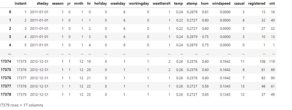

bk_dt.describe()

Description of integer columns of bike sharing dataset

bk_dt.info()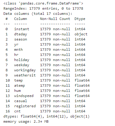

bk_dt.nunique()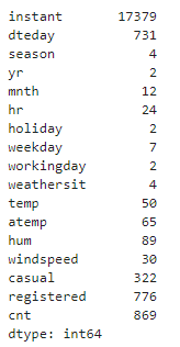

bk_dt.isnull().sum()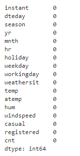

Rename the Columns

bk_dt = bk_dt.rename(columns = {'dteday' : 'Date','weathersit' : 'weather' , 'yr' : 'year', 'mnth' : 'month' , 'hr' : 'hour', 
                               'hum' : 'humidity' , 'cnt' : 'count'
                               })
bk_dt.head()

Renaming the column for better understanding

Change some variables datatype to category

# change int columns to category
cols = ['season','month','hour','holiday','weekday','workingday','weather']

for col in cols:
    bk_dt[col] = bk_dt[col].astype('category')
bk_dt.info()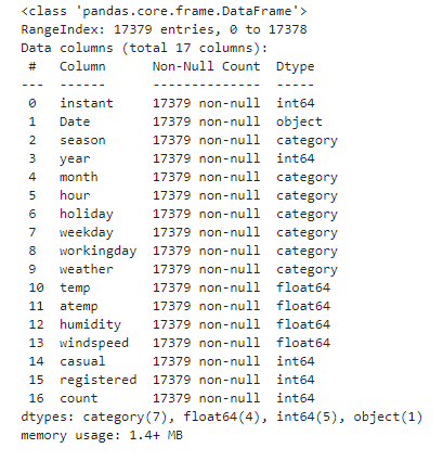

Convert to datetime

bk_dt['Date'] = pd.to_datetime(bk_dt['Date'])

Exploratory Data Analysis

If you want to learn about Exploratory data analysis, you can read my articles on EDA.

Time series analysis of bike rentals in a dataset

plt.figure(figsize=(12,6))
plt.plot(bk_dt['Date'], bk_dt['count'], label = 'Total Rentals')
plt.title('Bike Rentals over Time')
plt.xlabel('Date')
plt.ylabel('count')
plt.legend()
plt.show()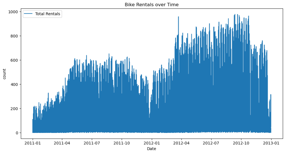

How many bike rentals in a hour

plt.figure(figsize=(12, 6))
sns.barplot(x='hour', y='count', data=bk_dt)
plt.title('Bike Rentals by Hour')
plt.xlabel('Hour')
plt.ylabel('Total Rentals')
plt.show()

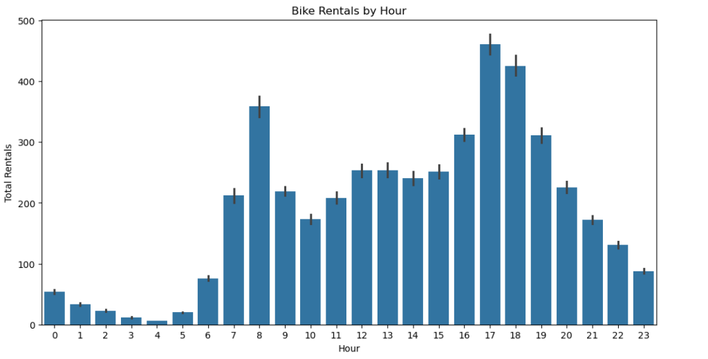
plt.figure(figsize = (12,6))
sns.pointplot(x = 'season', y = 'count', data = bk_dt)
plt.title('Total rentals by season')
plt.xlabel('Season')
plt.ylabel('Count')
plt.show()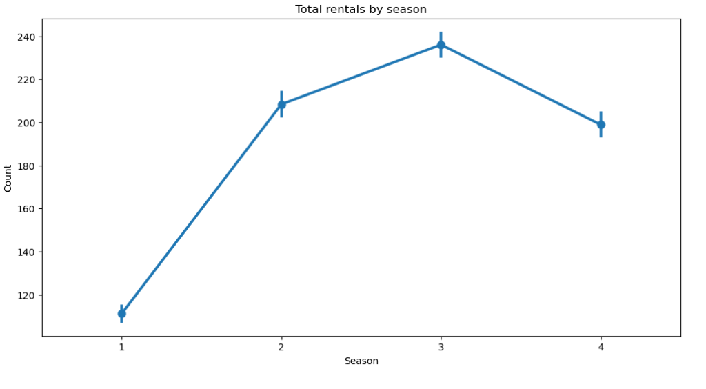

plt.figure(figsize = (15,10))
sns.heatmap(bk_dt.corr(), annot = True, cmap = 'coolwarm')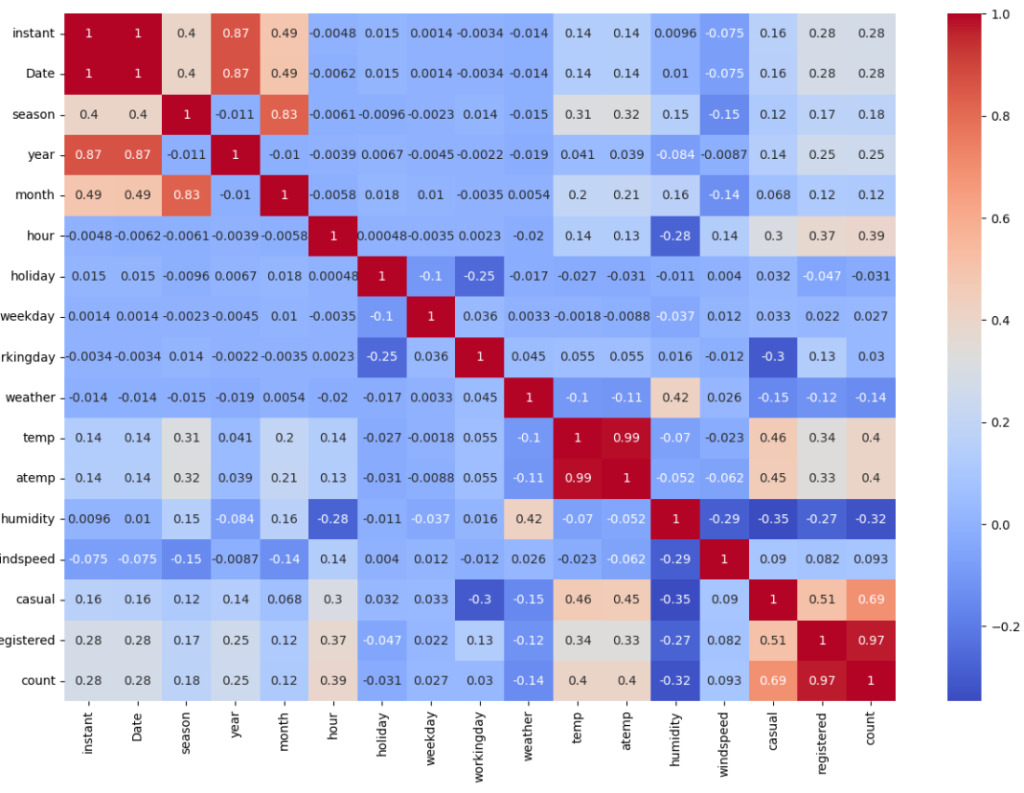

Heatmap analysis of bike sharing dataset

Feature Engineering: Convert categorical variables of the dataset into dummies

bk_dt = pd.get_dummies(bk_dt, columns=['season', 'month', 'hour', 'holiday', 'weekday', 'workingday', 'weather'], drop_first=True)
bk_dt.head()

Conversion categorical variables into dummy

Prepare data for modeling

X = bk_dt.drop(columns = ['Date', 'instant', 'casual', 'registered', 'count'])
y = bk_dt['count']

Splitting into training and testing

X_train, X_test, y_train, y_test = train_test_split(X, y, test_size = 0.3, random_state = 42)

Now we are going to apply machine learning algorithms

#Initialize the models

models = {
    'Linear Regression' : LinearRegression(),
    'Decision Tree Regressor' : DecisionTreeRegressor(random_state = 42),
    'Random Forest' : RandomForestRegressor(random_state = 42),
    'Gradient Boosting' : GradientBoostingRegressor(random_state = 42),
    'Support Vector' : SVR()
}

#Function to evaluate model 

def evaluate_model(model, X_train, y_train, X_test, y_test):
    model.fit(X_train, y_train)
    y_pred = model.predict(X_test)

    mae = mean_absolute_error(y_test, y_pred)
    mse = mean_squared_error(y_test, y_pred)
    rmse = np.sqrt(mse)
    r2 = r2_score(y_test, y_pred)

    return mae, mse, rmse, r2, y_pred

# Dictionary to store model performance
model_performance = {}
predictions = {}

# Evaluate all models
for name, model in models.items():
    mae, mse, rmse, r2, y_pred = evaluate_model(model, X_train, y_train, X_test, y_test)
    model_performance[name] = {'MAE': mae, 'MSE': mse, 'RMSE': rmse, 'R2': r2}
    predictions[name] = model.predict(X_test)

# Display model performance in a table
performance_df = pd.DataFrame(model_performance).T
performance_df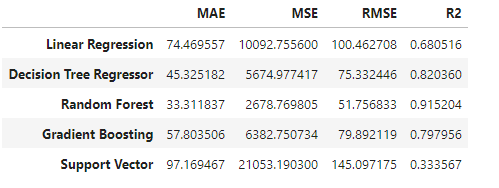

Visualize predictions vs actual values of all these 5 models

# Visualize predictions vs actual values
plt.figure(figsize=(20, 12))
for i, (name, preds) in enumerate(predictions.items(), 1):
    plt.subplot(3, 2, i)
    plt.scatter(y_test, preds, alpha=0.3)
    plt.plot([y_test.min(), y_test.max()], [y_test.min(), y_test.max()], '--r', linewidth=2)
    plt.title(f'{name}: Actual vs Predicted')
    plt.xlabel('Actual Values')
    plt.ylabel('Predicted Values')
plt.tight_layout()
plt.show()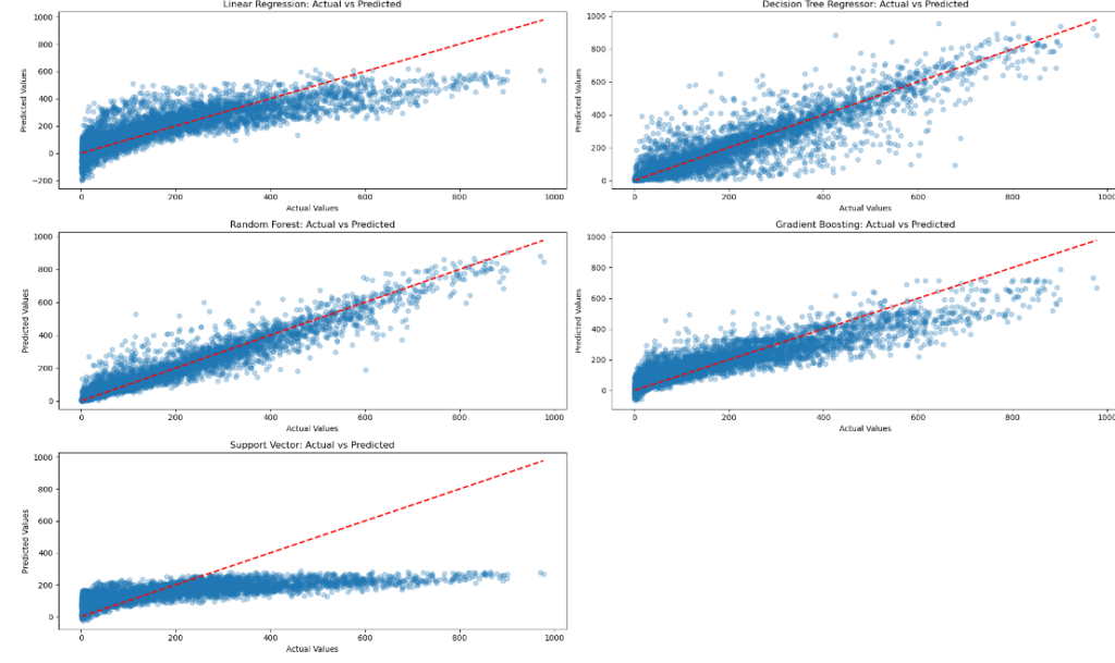

Visualize the regression algorithms prediction

From above graph Random Forest is the best model

# Visualize model performance
performance_df.plot(kind='bar', figsize=(15, 8))
plt.title('Model Performance Comparison')
plt.ylabel('Error')
plt.xticks(rotation=45)
plt.show()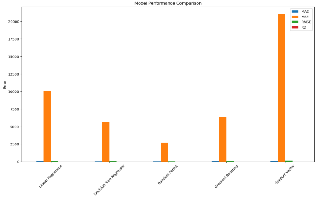

# Conclusion: Displaying the best performing model and its metrics
best_model = performance_df.sort_values(by='R2', ascending=False).iloc[0]
print("\nBest Performing Model:\n", best_model)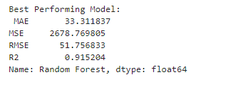

Hyperparameter Tuning (Random Forest) GridSearchCV

# Hyperparameter Tuning (Example: Random Forest)
param_grid = {
    'n_estimators': [100, 200, 300],
    'max_depth': [None, 10, 20, 30],
    'min_samples_split': [2, 5, 10]
}

rf_model = RandomForestRegressor(random_state=42)
grid_search = GridSearchCV(estimator=rf_model, param_grid=param_grid, cv=5, n_jobs=-1, verbose=2)
grid_search.fit(X_train, y_train)

# Best hyperparameters
print("Best Parameters:", grid_search.best_params_)

Best Parameters: {'max_depth': None, 'min_samples_split': 2, 'n_estimators': 300}


best_rf_model = grid_search.best_estimator_
mae, mse, rmse, r2, _ = evaluate_model(best_rf_model, X_train, y_train, X_test, y_test)
print(f"Random Forest - Tuned Model: MAE={mae}, MSE={mse}, RMSE={rmse}, R2={r2}")

Random Forest - Tuned Model: MAE=33.166340327628305, MSE=2649.6770998796947, RMSE=51.4750143261728, R2=0.9161251478072829